Real-Time Time-Dependent DMRG (RT-TD-DMRG)
References:
Ronca, E., Li, Z., Jimenez-Hoyos, C. A., Chan, G. K. L. Time-step targeting time-dependent and dynamical density matrix renormalization group algorithms with ab initio Hamiltonians. Journal of Chemical Theory and Computation 2017, 13, 5560-5571.
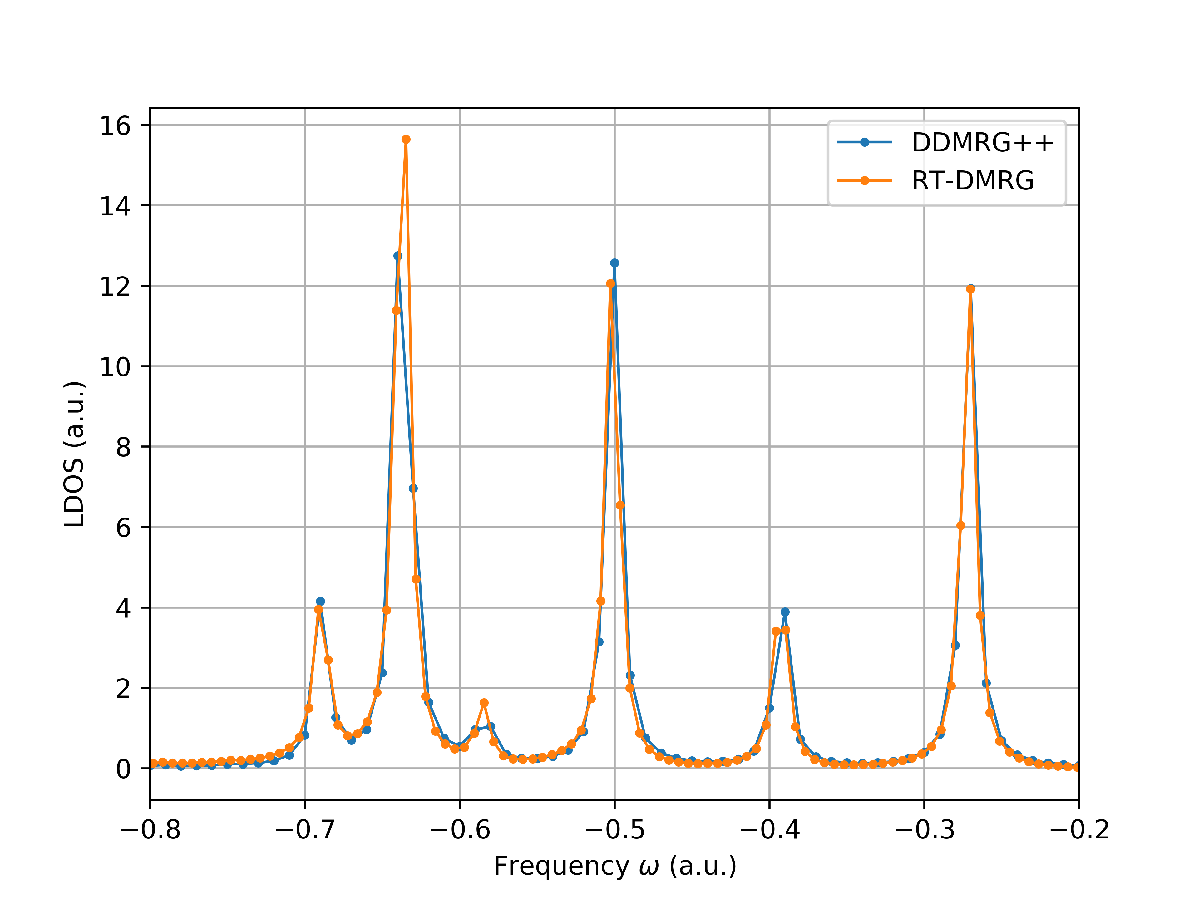
Here we use RT-TD-DMRG and Fast Fourier Transform (FFT) to calculate the same quantity defined in previous section, namely, the Green’s function for H10 (STO6G) (for a wide range of frequencies):
where \(|\Psi_0\rangle\) is the ground-state, \(i = j = 4\) (isite), \(\eta = 0.05\).
This is obtained from a Fourier transform from time domain to frequency domain:
where \(\mathrm{e}^{- \eta t}\) is a broading factor.
import time
import numpy as np
from pyblock3.algebra.mpe import MPE
from pyblock3.hamiltonian import Hamiltonian
from pyblock3.algorithms.core import DecompositionTypes
from pyblock3.fcidump import FCIDUMP
from pyblock3.symbolic.expr import OpElement, OpNames
from pyblock3.algebra.symmetry import SZ

np.random.seed(1000)
First, we load the definition of a quantum chemistry Hamiltonian from a FCIDUMP file.
Use flat = True to activate the efficient C++ backend.
fd = '../data/H10.STO6G.R1.8.FCIDUMP'
ket_bond_dim = 500
bra_bond_dim = 500

hamil = Hamiltonian(FCIDUMP(pg='d2h').read(fd), flat=True)
Then, we build the MPO mpo for the Hamiltonian. The compression of mpo can decrease
the MPO bond dimension, which will then save some runtime during DMRG and time evolution algorithms.
tx = time.perf_counter()
mpo = hamil.build_qc_mpo()
print('MPO (NC) =         ', mpo.show_bond_dims())
print('build mpo time = ', time.perf_counter() - tx)

tx = time.perf_counter()
mpo, _ = mpo.compress(left=True, cutoff=1E-9, norm_cutoff=1E-9)
print('MPO (compressed) = ', mpo.show_bond_dims())
print('compress mpo time = ', time.perf_counter() - tx)
Now we build a random MPS, as the initial guess for the DMRG algorithm.
mps = hamil.build_mps(ket_bond_dim)
print('MPS = ', mps.show_bond_dims())
MPE (Matrix Product Expectation) is a bra-mpo-ket tensor network structure,
with some partial contraction of envionments stored internally.
DMRG (sweep) algorithm can be invoked based on MPE.
For DMRG algorithm, bra and ket are the same, both represented as the mps object.
bdims = [500]
noises = [1E-4, 1E-5, 1E-6, 0]
davthrds = None

dmrg = MPE(mps, mpo, mps).dmrg(bdims=bdims, noises=noises,
                            dav_thrds=davthrds, iprint=2, n_sweeps=20, tol=1E-12)
ener = dmrg.energies[-1]
print("Energy = %20.12f" % ener)
Now ener is the ground-state energy \(E_0\) of the system. We substract
this constant from MPO to let the mpo object represent \(\hat{H}_0 - E_0\).
isite = 4
mpo.const -= ener
Here, dop is the destruction operator \(\hat{a}_{4\alpha}\), defined using OpElement,
where the first argument OpNames.D is the operator name,
the second argument (isite, 0) is the orbital index (counting from zero) and spin index (0 = alpha, 1 = beta),
and the last argument q_label is a quantum number, representing how this operator changes
the quantum number of a state. Here \(\hat{a}_{4\alpha}\) will decrease particle number by 1,
decrease 2S_z by 1, and change point group irrep by the point group irrep of orbital isite (which is 4 here).
An MPO dmpo (bond dimension = 1) can be directly built from single site operator dop using
hamil.build_site_mpo().
dop = OpElement(OpNames.D, (isite, 0), q_label=SZ(-1, -1, hamil.orb_sym[isite]))
dmpo = hamil.build_site_mpo(dop)
print('DMPO =         ', dmpo.show_bond_dims())
Next, we need to construct an MPS bra, which is \(\hat{a}_{4\alpha} |\Psi_0\rangle\) where
\(|\Psi_0\rangle\) is the ground-state mps.
First we define bra as a random MPS with the correct quantum number.
The quantum number of bra is simply the sum of the quantum number of dop and mps.
bra = hamil.build_mps(bra_bond_dim, target=SZ.to_flat(
    dop.q_label + SZ.from_flat(hamil.target)))
Then we use MPE.linear() to fit bra to dmpo @ mps.
This is a sweep algorithm similar to DMRG.
In principle, the following line (and the above line) can be replaced by simply
bra = dmpo @ mps; bra.fix_pattern() (which may be slower).
Also note that MPE.linear may have some problems handling the constant term in MPO.
If the mpo has a constant term (the dmpo here does not have a constant), one can do
MPE(bra, mpo - mpo.const, mps).linear(...); bra += mpo.const * mps.
MPE(bra, dmpo, mps).linear(bdims=[bra_bond_dim], noises=noises,
                                cg_thrds=davthrds, iprint=2, n_sweeps=20, tol=1E-12)
Now we obtain a (deep) copy of bra to be ket. Later when we time evolve ket,
bra will not be changed.
ket = bra.copy()
dt = 0.1
eta = 0.05
t = 100.0

nstep = int(t / dt)
Real time evolution can be performed using MPE.tddmrg(), with a imaginary dt argument.
normalize should be set to False, so that we will not keep ket normalized,
so that the constant prefactor in ket will transformed into rtgf, which is convenient.
Note that since (in principle) real time evolution does not change the norm of the MPS,
whether keeping the MPS normalized should not make a difference.
When MPS is not explicitly normalized, the norm of MPS printed after each sweep can be
used as an indicator of the accuracy of the algorithm.
For imaginary time evolution, however, it is recommended to explicitly normalize MPS,
since during the imaginary time evolution the prefactor in the MPS is not a constant.
It can grow up rapidly, which may create some numerical problem.
After each time step, the overlap between bra and ket, which is \(G_{44}(t)\), is calculated
and stored in rtgf.
mpe = MPE(ket, mpo, ket)
rtgf = np.zeros((nstep, ), dtype=complex)
print('total step = ', nstep)
for it in range(0, nstep):
    cur_t = it * dt
    mpe.tddmrg(bdims=[500], dt=-dt * 1j, iprint=2, n_sweeps=1, n_sub_sweeps=2, normalize=False)
    rtgf[it] = np.dot(bra.conj(), ket)
    print("=== T = %10.5f EX = %20.15f + %20.15f i" % (cur_t, rtgf[it].real, rtgf[it].imag))
A single step of time evolution can also be written as (currently not completely supported),
which can be significantly slower than MPE.tddmrg().
# fmps = rk4_apply((-dt * 1j) * mpo, mps)
Finally, one can use FFT to transform back to frequency domain.
def gf_fft(eta, dt, rtgf):

    dt = abs(dt)
    npts = len(rtgf)

    frq = np.fft.fftfreq(npts, dt)
    frq = np.fft.fftshift(frq) * 2.0 * np.pi
    fftinp = -1j * rtgf * np.exp(-eta * dt * np.arange(0, npts))

    Y = np.fft.fft(fftinp)
    Y = np.fft.fftshift(Y)

    Y_real = Y.real * dt
    Y_imag = Y.imag * dt

    return frq, Y_real, Y_imag

frq, yreal, yimag = gf_fft(eta, dt, rtgf)
The following figure compares the results obtained from DDMRG++ and td-DMRG (with lowdin orbitals, dt = 0.1, eta = 0.005, t = 1000.0).